• View
• Edit
• History
• Print

Knowledge gaps and recent progress

Chapter 3. Phenomena Relevant to Accidents

All materials deform under load. The stress which a structural material is able to withstand is conditioned by its ductility that is the ability to deform permanently prior to fracture. A material is elastic if, after being elongated under stress, it returns to its original shape as soon as the stress is removed. Elastic deformation is recoverable and involves both a change of shape and volume. At a certain strain, when the load exceeds the yield stress, the stress strain behaviour becomes non-linear and the material will retain a permanent deformation. A further increase of the strain eventually reaches the ultimate load called ‘tensile stress’ beyond which the stress decreases finally leading to rupture. Ductile materials can accommodate local stress concentrations, they can be greatly bent and reshaped without breaking. In contrast, brittle materials have only a small amount of elongation at fracture. The strength of ductile material is approximately the same in tension and compression, whereas that of brittle material is much higher in compression than it is in tension. Brittle materials do not show the phase of permanent elongation. They fail suddenly and catastrophically when they are exposed to tensile stress

Hydrogen can have two main damaging effects on materials:

- Low temperature effect. At low temperature for example, when it is stored in liquid form, it can have an indirect effect called “cold embrittlement”. This effect is not specific to hydrogen and can occur with all the cryogenic gases if the operating temperature is below the ductile-brittle transition temperature. Cryogenic temperatures can affect structural materials. With decreasing temperature, there is a decrease in toughness that is very slight in face centred cubic materials, but can be very marked in body centred cubic ones such as ferritic steels. Metals that work successfully at low temperatures include aluminium and its alloys, copper and its alloys, nickel and some of its alloys, as well as stable austenitic stainless steels.

– Hydrogen embrittlement. Hydrogen can have a direct effect on the material by degrading its mechanical properties; this effect is called “hydrogen embrittlement” and is specific to the action of hydrogen and some other hydrogenated gases. Hydrogen has to breakdown from its molecular into the atomic form in order to be able to enter the material and to produce the deleterious effect on its properties.

The effect of hydrogen on material behaviour, on its physical properties, is a fact. Hydrogen may degrade the mechanical behaviour of metallic materials and lead them to failure. Hydrogen embrittlement affects the three basic systems of any industry that uses hydrogen: Production, Transport/ Storage and Use.

When tensile stresses are applied to a hydrogen embrittled component, it may fail prematurely in an unexpected and sometimes catastrophic way. An externally applied load is not required as the tensile stresses may be due to residual stresses in the material. The threshold stresses to cause cracking are commonly below the yield stress of the material. Thus, catastrophic failure can occur without significant deformation or obvious deterioration of the component.

It can take place in two different ways:

– Internal Hydrogen Embrittlement. Takes place when hydrogen enters the metal during its processing. It is a phenomenon that may lead to the structural failure of material that never has been exposed to hydrogen before. Internal cracks are initiated showing a discontinuous growth. Not more than 0.1 - 10 ppm hydrogen in the average are involved. The effect is observed in the temperature range between 173 and 373 K and is most severe at near room temperature.

– External Hydrogen Embrittlement. Occurs when the material is subjected to a hydrogen atmosphere, e.g. storage tanks. Absorbed and/or adsorbed hydrogen modifies the mechanical response of the material without necessarily forming a second phase. The effect strongly depends on the stress imposed on the metal. It also maximizes at around room temperature. The hydrogen that has entered the material can be either in interstitial solid solution state or in a combined state forming H2, CH4 or hydrides. When hydrogen is dissolved in the material as interstitial solid solution promoting lattice decohesion, the phenomenon is called «gaseous hydrogen embrittlement». It takes place generally at temperatures close to ambient and the transport of the hydrogen occurs mainly by the net dislocations when the material is undergoing deformation. When hydrogen is present in a combined state, it is a matter of «hydrogen attack». It is a phenomenon in which the hydrogen chemically reacts with a constituent of the metal to form a new microstructural element or phase. The hydrogen can react with the carbon of the alloy to form molecules of methane; this leads to the formation of micro-cavities and to a lack of carbon in the alloy. Atomic hydrogen can also recombine forming hydrogen molecules. Hydrogen can react with a specific element forming hydrides precipitating in a new phase. In all these cases, hydrogen is transported mainly by diffusion and the phenomenon is increased with the temperature. The case of hydride formation in titanium alloys is a typical one. The microstructure of these alloys consists usually of two phases with different hydrogen solubility and diffusivity. Hydrogen enters the alloy via grain boundaries or other easy paths as beta phase, forming hydrides that precipitate in the alfa phase.

Materials

Material suitability for hydrogen service should be evaluated carefully before it is used. A material should not be used unless data are available to prove that it is suitable for the planned service conditions. In case of any doubt the material can be subjected to hydrogen embrittlement susceptibility testing (e.g. ISO 11114-4).

According to the information included in the ISO/TR 15916:2004 Basic considerations for the safety of hydrogen systems /Technical Report most of the metallic materials present a certain degree of sensitivity to hydrogen embrittlement. However, there are some that can be used without any specific precautions as for example brass and most of the copper alloys, aluminium and its alloys and austenitic stainless steel. On the other hand, nickel and high nickel alloys or titanium and its alloys are known to be sensitive to hydrogen embrittlement. For steels the sensitivity may depend on several factors as the exact chemical composition, heat or mechanical treatment, microstructure, impurities and strength. Concerning non-metallic materials, ISO/TR 15916:2004 also provides information as far as the suitability of some selected materials.

Fortunately many materials can be safely used under controlled conditions ( e.g. limited stress , absence of stress raisers such as surface defects….).

Sources and references: Dechema, A 1987, ‘Study for the Generation, Inter-Continental Transport, and Use of Hydrogen as a Source of Clean Energy on the Basis of Large-Scale and Cheap Hydro-Electricity’. Final Report on Contract Nº. EN3S-0024-D(B), Deutsche Gesellschaft für Chemisches Apparatewesen. Frankfurt. American National Standard 1990, Steels for Hydrogen Service at Elevated Temperatures and Pressures in Petroleum Refineries and Petrochemical Plants. ANSI/API 941-1990. ‘Materiales en la tecnología del hidrógeno’ by UPM, Madrid. <http://www.energiasostenible.net/materiales_hidrogeno.htm> Tzimas, E, Filiou, C, Peteves, SD, Veyret, JB, (ed.) 2003, Hydrogen Storage: State Of The Art and Future Perspective, European Commission - Directorate General Joint Research Centre (DG JRC) -Institute for Energy. Petten. Edeskuty, FJ, Stewart, WF (ed.) 1996, Safety in Handling of Cryogenic Fluids. The International Cryogenics Monograph Series, Plenum Press. New York. Kussmaul, K, Deimel, P 1995, Materialverhalten in H2-Hochdrucksystemen, VDI Berichte Nº. 1201, VDI-Verlag, Düsseldorf. Mohitporu, M, Pierce, CL, Graham, P 1990, Design Basis Developer for H2 Pipeline. Oil & Gas Journal. 28 May. Louthan, MR, Morgan, MJ 1996, Some Technology Gaps in the Detection and Prediction of Hydrogen-Induced Degradation of Metals and Alloys. J. Nondestructive Evaluation 15. Barthélémy, H 2006, ‘Compatibility of metallic materials with hydrogen. Review of the present knowledge’. Proceedings of the 16th World Hydrogen Energy Conference, Lyon 13-16 June 2006. International Organization for Standarization 2004, Basic considerations for the safety of hydrogen systems /Technical Report, ISO/TR 15916:2004. First edition 2004-02-15. Verfondern, K (ed) 1999, Hydrogen as an energy carrier and its production by nuclear power (IAEA-TECDOC-1085). International Atomic Energy Agency. Barthélémy, H 1989, ‘How to Select Steel for Compressed and Liquefied Hydrogen Equipment, Instrumentation of Steels with hydrogen in petroleum industry pressure vessel service’. Proceeding of the Industrial Conference Paris. Barthélémy, H, Château, G. 1988, ‘Hydrogen embrittlement of low alloyed ferritic steels by hydrogen and hydrogen sulfide under high pressure’. Proceedings of Hydrogen and Materials. Beijing. Azkarate, I 1992, ‘Corrosión bajo factores mecánicos asistida por hidrógeno de aleaciones de titanio’, PhD thesis, Instituto Químico de Sarriá, Universidad Ramón Llull, Barcelona. Azkarate, I, Erauzkin, E, Pelayo, A, Irisarri, A.Mª 1988, ‘Fragilización por hidrógeno de tubos de acero API5 LX-52 y X-60’, Rev. Metalurgia. Vol. 24 (5), 331-336. Barthélémy, H 2004, ‘Learning from gas cylinders incidents. A general overview’, Proceedings of the 14TH Symposium EIGA : Packaged gases : past, present and future. Strasbourg. Barthélémy, H 1990 ‘Behavior of steel in the presence of pressurized hydrogen. Recommendation for the construction of pressurized equipment’,. Proceedings of the Third meeting on inspection in the Chemical Industry, Chemical Industry Union, Marseille, France.

And thanks to Sandia National Laboratories and especially to Mr. Moen and Drs. Somerday and San Marchi for their contribution to this chapter.

• Hydrogen Release

Contributing Authors

Contributing author	Main contributions	Organisation
A.G.Venetsanos	Chapter coordinator	NCSRD
P. Benard and A.G. Venetsanos	Subsonic and sonic jets	UQTR, NCSRD
A.G.Venetsanos and E. Papanikolaou	Two phase jets	NCSRD
K. Verfondern	LH2 pool spreading and vaporization	FZJ
A.G. Venetsanos and P. Adams	Other types of releases	NCSRD, VOLVO

Contributing reviewer	Organisation
O.R. Hansen	GEXCON

---

Hydrogen Release

Subsonic

Gaseous hydrogen releases through a hole or a conduct are produced as a result of a positive pressure difference between a container and its environment. The aperture is often modeled as a nozzle. Depending on the upstream pressure, a flow through a convergent nozzle to a lower downstream pressure can either be chocked (or sonic) or subsonic. The crossover pressure is a function of the ratio of the constant volume to the constant pressure specific heat, see Hanna and Strimaitis (HannaSR:1989).

The flow resulting from a subsonic release is basically an expanded jet. The concentration profile of hydrogen in this expanded jet is inversely proportional to the distance to the nozzle along the axis of the jet. At a given distance from the nozzle, the concentration profile of hydrogen in air is distributed according to a Gaussian function centered on the axis. The following formula has been suggested by Chen and Rodi (ChenCJ:1980) for the axial concentration (v/v) decay of variable density subsonic jets:

{{C(x)} \over {C_j }} = K{{d_{j} } \over {x - x_0 }}\left( {{{\rho _\alpha } \over {\rho _g }}} \right)^{1/2}

(1)

Where C(x) is the concentration (vol) at location x, C_j is the concentration at the outlet nozzle, d_j is the jet discharge diameter, ρ_α is the density of the ambient air, ρ_g the density of the gas at ambient conditions, x is the distance from the nozzle along the jet axis, x₀ is the virtual absicca of the hyperbolic decrease (usually neglected because it is of the order of magnitude as the real diameter) and K is a constant equal to 5.

For hydrogen, chocked releases occur when the upstream pressure is 1.9 times larger than downstream, otherwise the flow is subsonic. The flow rate of a chocked flow is only a function of the upstream pressure, whereas the flow rate of a subsonic release will depend on the difference between the upstream and downstream pressures. A release from a compressed gas storage system into the environment will therefore be chocked as long as the storage pressure remains larger than 1.89 bars.

A chocked release of hydrogen undergoes a pressure and a temperature drop at the exit of the nozzle. The pressure will drop until the exit pressure reaches the value of the downstream pressure. At that point, the release becomes subsonic and the exit pressure remains constant at the downstream value. In the chocked regime, the gas velocity at the exit of the nozzle is exactly the sonic velocity of the gas. The flow rate can therefore be estimated from

\dot m = \rho Ac

(2)

where ρ is the density of hydrogen at the exit of the nozzle, calculated using the local value of the temperature and the pressure. The flow rate will also be affected by the shape of the aperture, friction and the length of the conduit between the reservoir and the release point.

Because the exit density changes as a function of temperature and pressure, and because the sonic velocity is essentially proportional to the square root of the temperature, the flow rate will not remain constant but will vary as the upstream pressure drops (Fig. 1).

Figure 1 shows the effect of using real gas hydrogen properties compared to ideal gas. It is well known that at high storage pressures real hydrogen gas densities are lower than ideal gas densities. Table 1 compares real versus ideal hydrogen densities at temperature 288 K and pressures 200 and 700 bar, (values taken from the (MarshallN:1976) ). For given storage volume the real gas assumption results in less stored hydrogen mass and consequently less released mass in an accidental situation.

Table 1: Comparison between real and ideal gas properties

Pressure (bar)	Real density (kg m-3)	Ideal density (kg m-3)	Relative error (%)
200	14.96	16.85	12.6
700	40.18	58.90	46.6

The effect of real gas properties has been taken into account in the 1983 Stockholm hydrogen accident simulations by Venetsanos et al.(VenetsanosAG:2003), where tables from Encyclopedie des gaz were used to obtain the hydrogen density. Real gas properties calculations based on the Beattie–Bridgeman equation of state were reported by Mohamed and Paraschivoiu (MohamedK:2005) , who modeled a hydrogen release from a high pressure chamber. Real gas properties using the Abel-Nobel equation of state were considered by Cheng et al.(ChengZ:2005) who performed hydrogen release and dispersion calculations for a hydrogen release from a 400 bar tank through a 6 mm PRD opening and found that the ideal gas law overestimates the hydrogen release rates by up to 35% during the first 25 seconds after the release. Based on these findings these authors recommended a real gas equation of state to be used for high pressure PRD releases.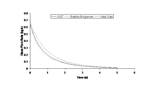

Fig. 1: Mass flow rate as a function of time from a 6 mm aperture of a 345 bar compressed gas 27.3 litre cylinder (calculated using the NIST (LemmonEW:2000) , the Bettie-Bridgeman and the ideal gas equations of state based on (MohamedK:2005).

A chocked jet (Fig. 2) can be basically divided into an under-expanded region, where the flow becomes supersonic, forming a cone-like structure (the Mach cone) (Fig. 3); and an expanded region, which behaves similarly to an expanded subsonic jet. The under-expanded region is characterized by a complex shock wave pattern, involving bow and oblique shocks (Figs 3 and 4).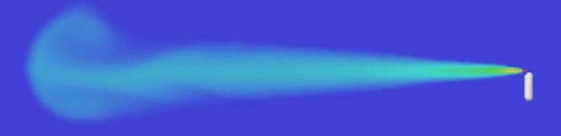

Fig. 2: Chocked release from a 150 litre 700 bar reservoir (AngersB:2006).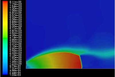

Fig. 3: Under-expanded chocked release of hydrogen (the Mach number is calculated with respect to air).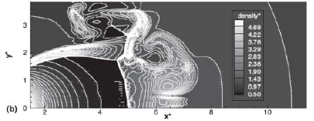

Fig. 4: Normalized density contours as a function of position (hydrogen jet in hydrogen atmosphere; source: (PedroG:2006)

As for subsonic releases, the concentration profile of hydrogen in the expanded region is inversely proportional to the distance to the nozzle along the axis of the jet and is distributed according to a Gaussian function at a fixed distance from the nozzle. The axial concentration decay can be calculated using the formula for variable density subsonic jets, see Eq.(1), where the discharge diameter is replaced by the effective diameter, which is representatve of the jet diameter at the start of the subsonic region, i.e. after the Mach cone.

{{C(x)} \over {C_j }} = K{{d_{eff} } \over {x - x_0 }}\left( {{{\rho _\alpha } \over {\rho _g }}} \right)^{1/2}

(3)

For the determination of the effective diameter various approaches have been proposed, such as (BirchAD:1984), (EwanBCR:1986) and (BirchAD:1987). In this latest approach, the effective diameter and corresponding effective velocity is calculated by applying the conservation of mass and momentum, between the outlet and a position beyond the Mach cone where pressure first becomes equal to the ambient, assuming no entrainment of ambient air.

d_{eff} = \left( {{{\rho _j u_j } \over {\rho _g u_{eff} }}} \right)^{1/2} d_j

(4)

Where ρ_j and u_j are the density and the velocity of the jet at the outlet (respectively), ueff is the effective velocity, d_j the diameter of the outlet. The effective velocity is calculated using the following expression:

u_{eff} = u_j + {{p_j - p_\alpha } \over {\rho _j u_j }}

(5)

where p_j is the pressure of the jet at the outlet and p_α is the ambient pressure.

Regarding the constant K entering Eq.(3), different values have been reported in the literature. An average value of 4.9 is mentioned by Birch (BirchAD:1984) . An average value of 5.4 was reported in (BirchAD:1987) . This approach ((BirchAD:1984) and (BirchAD:1987) ; (HoufW:2005)) has been validated experimentally for vertical chocked releases for pressures below 70 bars for natural gas and hydrogen.

A lower value K = 3.7 was reported by Ruffin (RuffinE:1996) who investigated experimentaly the concentration field of horizontal supercritical jets of methane and hydrogen for 40 bars storage pressure and with orifice diameters in the range from 25 to 150 mm. Ruffin et al. used the Birch approach (BirchAD:1984) in defining the effective diameter. Furthermore, Chaineaux (ChaineauxJ:2006) referring to the experiments in (ChaineauxJ:1999) reported a value of 2.25 for 200 bar hydrogen release from a 0.5 mm hole and a value of 2.89 for 700 bar hydrogen release from a 0.35 mm hole.

Other experiments supporting the decay law of Eq.(3) are the experiments by Chitose et al. (ChitoseK:2006) who have measured the concentration profile of a hydrogen release from a 40 MPa storage unit. They observed that as a function of distance, the concentration profile of leaks with diameters ranging from 0.25 to 2 mm was inversely proportional to the distance to the nozzle and that all data points fell on a simple inverse power scaling law as a function of the normalized distance. Based on the experimental work, they obtained flammable concentration extents of 2.6 m, 6.6 m and 13.4 m for leak diameters of 0.2, 0.5 and 1.0 mm respectively. An experiment to measure the concentration profile of a horizontal release using a 10 mm diameter leak through a broken pipe from a 40 MPa storage unit showed that the extent of the 4% (vol) concentration envelope reached a distance of about 18 meters, 3 seconds after release.

Flammable release extents can approximately be calculated using Eq.(3). The maximum extent of a time-dependent release will not be estimated using the initial storage pressure, but using a later value (see Houf and Schefer, (HoufW:2005)). Predicted flammable release extents are shown in Fig. 5 below. The axial distance to the lower flammability limit of 4% (vol) for hydrogen varies from 2 to 53 m for leak diameters ranging from 0.25 mm to 6.35 mm if the storage pressure is 1035 bars.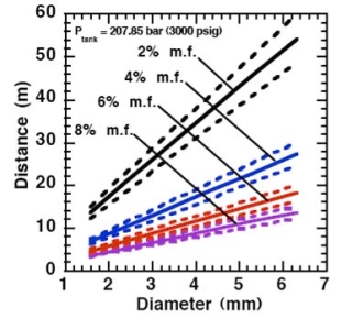

Fig. 5: Distances to concentrations of 2.0%, 4.0%, 6.0%, and 8.0% mole fraction on the centreline of a jet release from a 207.85 bars tank for various leak diameter obtained using the Sandia/Birch approach. The dashed lines indicate upper and lower bounds with ±10% uncertainty in the value of the constant K. (from (HoufW:2007))

References

LIST,NS

---

Hydrogen Release

Two phase jets

The phenomena associated with two phase jet dispersion are reviewed by Bricard and Friedel (BricardP:1998). Within a short distance just downstream from the outlet, the flow can experience drastic changes which must be considered for subsequent dispersion calculations. The physical phenomena taking place in this region comprise (i) flashing if the liquid is sufficiently superheated, (ii) gas expansion when the flow is choked and (iii) liquid fragmentation. The corresponding quantities to be determined as initial conditions for subsequent dispersion calculations are the flash fraction, the jet mean temperature, velocity and diameter, and the droplet size.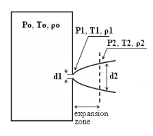

Fig. 1: Model of a two-phase flashing jet

Flashing occurs when the liquid is sufficiently superheated at the outlet with respect to atmospheric conditions and corresponds to the violent boiling of the jet. The vapour mass fraction after flashing is most often determined in the models by assuming isenthalpic depressurization of the mixture between the outlet (position 1 in Fig. 1) and the plane downstream over which thermodynamic equilibrium at ambient pressure is attained (position 2 in Fig. 1):

$$ x_2 = {{\int\limits_1^2 {C_{pf} dT} } \over {H_{fg} }} $$

(1)

Where H_fg is the latent heat of vaporization and C_pf is the liquid specific heat.

When the flow is choked at the outlet, the gas phase expands to ambient pressure within a downstream distance of about two orifice diameters. This causes a strong acceleration of the two-phase mixture and usually an increase of the jet diameter. In the models, the velocity and diameter of the jet at the end of the expansion zone are given by the momentum and mass balance, respectively, integrated over a control volume extending from the outlet (position 1) to the plane where atmospheric pressure is first reached (position 2). It is assumed that no air is entrained in this region. The approach is similar to the one described above for choked gaseous hydrogen jets. The corresponding equations according to Fauske and Epstein (FauskeHK:1988) are:

$$ d_2 = d_1 \left( {{{\rho _1 u_1 } \over {\rho _2 u_2 }}} \right)^{1/2} ,{\kern 1pt} {\kern 1pt} {\kern 1pt} {\kern 1pt} {\kern 1pt} u_2 = u_1 + {{P_1 - P_2 } \over {\rho _1 u_1 }} $$

(2)

Liquid fragmentation (or atomization) is caused by two main physical mechanisms: flashing and aerodynamic atomization. With flashing atomization, the fragmentation results from the violent boiling and bursting of bubbles in the superheated liquid, whereas aerodynamic atomization is the result of instabilities at the liquid surface. The determination of the initial droplet size (position 2) is a required initial condition, if the subsequent dispersion models account for fluiddynamic and thermodynamic non-equilibrium phenomena, like rainout and/or droplet evaporation. In the case of aerodynamic fragmentation, the maximum stable drop size is usually given by a critical Weber number, which represents the ratio of inertia over surface tension forces:

$$ We_{\max } = {{\Delta U^2 \rho _g d_{\max } } \over \sigma } $$

(3)

Where σ is the surface tension of the liquid, ρ_g is the gas density, d_max is maximum stable droplet diameter and ΔU the mean relative velocity between both phases. A range of values are used for the maximum Weber number, see (BricardP:1998) with 12 being the most common value.

In the previous discussion the mass flow rate and outlet conditions (position 1) were assumed known. Hanna and Strimaitis (1989)(HannaSR:1989) have reviewed various approaches for calculating the release mass flow rate for liquid and two-phase flow releases. Detailed information on the subject can be found in chapter 15 of Lees (LeesFP:1996a) , in chapter 9 of Etchells and Wilday (EtchellsJ:1998) as well as in the older review of critical two phase flow models by D’Auria and Vigni (DAuriaF:1980) If the liquid in the reservoir is at saturated conditions, and if equilibrium flow conditions are established (i.e. for outflow pipe lengths > 0.1 m) then the two-phase choked mass flux (kg s^-1 m^-2) can be calculated following Fauske and Epstein (FauskeHK:1988):

$$ G = {{H_{fg} } \over {v_g - v_f }}\left( {{1 \over {C_{pf} T}}} \right)^{1/2} $$

(4)

Where H_fg is the latent heat of vaporization, C_pf is the liquid specific heat, T is the saturation temperature which is function of the storage pressure p, v_g, v_f are the saturated vapour and liquid specific volumes. This equation applies only if the vapor mass fraction after depressurization to atmospheric pressure (position 2) obeys the following criterion:

$$ x_2 < {{p\left( {v_g - v_f } \right)\left( {C_{pf} T} \right)} \over {H_{fg}^2 }} $$

(5)

Figure 2 shows the equilibrium choked mass flux calculated using Eq. (4) for an LH₂ release as function of the storage pressure.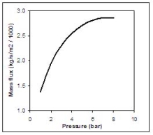

Fig. 2: Mass flux calculated using Eq. (4) for an LH₂ release, as function of the storage pressure

References

Invalid BibTex Entry!

---

Hydrogen Release

Buoyant jets and plumes

After the hydrogen-rich cloud losses its inertia, buoyant forces become more and more dominant. Usually, this cloud is less dense than the surrounding air and then the buoyancy force is directed upwards. When the hydrogen released is very cold, buoyant forces could point downwards. However, the heat and mass transfers during the mixing process reduce the mixture density and invert the buoyant force direction. The fluid structure established is a plume, where two regions are distinguished: forced plumes and buoyant plumes. At the forced plume both forces (inertia and buoyancy) are of similar magnitude and separate pure inertia region (jet) apart from the pure buoyant region (plume).

The buoyancy to inertia ratio is expressed by the densimetric Froude number:

Fr = {{\rho_0 U_0^2} \over {(\rho_\infty - \rho_0 )gd_0}}

(1)

{\omega} = {{\rho _\infty} \over {\rho _0}}

(2)

{L_{Mo}} = Fr^{1/2}{\omega}^{-1/4}d_0

(3)

where U₀, ρ₀ and d₀ are the fluid velocity, the fluid density and the diameter at the break point, respectively, g is the gravity acceleration and ρ_∞ is the bulk density. Using this dimensionless number, (GebhartB:1988) recommend the following expressions (Tab. 1) for the three regions of a vertical upward structure. The x-direction is along the centreline of the structure, u_c, ρ_c and c_c the fluid velocity, the fluid density, and concentration at the centreline. Notice that velocity (u) and concentration (c) profiles at any transversal plane are expressed by Gaussian functions.

When the structure shape is very different from an upward vertical one, these regions need to be established by numerical simulations.

Table 1: Recommended expressions for the three regions of a vertical upward structure from (GebhartB:1988).

Regions	INERTIA	INTERMEDIUM	BOUYANCY
STRUCTURE	JET	FORCED PLUME (OR BUOYANT JET)	BUOYANT PLUME
BOUNDS	$$ {x \over L_{Mo}} < 0.5 $$	$$ 0.5 \le {x \over L_{Mo}} \le 5 $$	$$ 5 < {x \over L_{Mo}} $$
$$ {{u_c } \over {U_0 }} $$	$$ 6.2 {\omega}^{1/2}\left({x \over {d_0 }}\right)^{- 1} $$	$$ 7.26Fr^{ -1/10} {\omega}^{-9/20} \left( {{x \over {d_0 }}} \right)^{ - 4/5} $$	$$ 3.5Fr^{ -1/3} {\omega}^{-1/3} \left( {{x \over {d_0 }}} \right)^{ - 1/3} $$
$$ {{(\rho _\infty - \rho _c )} \over {(\rho _\infty - \rho _0 )}} $$	$$ 5{\omega}^{1/2} \left( {{x \over {d_0 }}} \right)^{ - 1} $$	$$ 4.4Fr^{1/8} {\omega}^{7/16} \left( {{x \over {d_0 }}} \right)^{-5/4} $$	$$ 9.35Fr^{1/3} {\omega}^{1/3} \left( {{x \over {d_0 }}} \right)^{-5/3} $$
$$ {{c_c } \over {C_0 }} $$	$$ 6.34\left( {{x \over {d_0 }}} \right)^{ - 1} $$	--	$$ 12.16Fr^{1/3} {\omega}^{-1/3} \left( {{x \over {d_0 }}} \right)^{ - 5/3} $$
$$ {u \over {u_c }} $$	$$ \exp \left[ { - 92\left( {{r \over x}} \right)^2 } \right] $$	--	$$ \exp \left[ { - 90\left( {{r \over x}} \right)^2 } \right] $$
$$ {c \over {c_c }} $$	$$ \exp \left[ { - 52\left( {{r \over x}} \right)^2 } \right] $$	--	$$ \exp \left[ { - 80\left( {{r \over x}} \right)^2 } \right] $$

References

Invalid BibTex Entry!

LH

Liquefied gases are characterized by a boiling point well below the ambient temperature. If released from a pressure vessel, the pressure relief from system to atmospheric pressure results in spontaneous (flash) vaporization of a certain fraction of the liquid. Depending on leak location and thermodynamic state of the cryogen (pressure expelling the cryogen through the leak is equal to the saturation vapour pressure), a two-phase flow will develop, significantly reducing the mass released. It is connected with the formation of aerosols, which vaporize in the air without touching the ground. Conditions and configuration of the source determine features of the evolving vapour cloud such as cloud composition, release height, initial plume distribution, time-dependent dimensions, or energy balance. The phenomena that may occur after a cryogen release into the environment are shown in Fig. 1.

Fig. 1: Physical phenomena occuring upon the release of a cryogenic liquid

LH₂ Vaporization

The release as a liquefied gas usually results in the accumulation and formation of a liquid pool on the ground, which expands, depending on the volume spilled and the release rate, radially away from the releasing point, and which also immediately starts to vaporize. The equilibrium state of the pool is determined by the heat input from the outside like from the ground, the ambient atmosphere (wind, insolation from the sun), and in case of a burning pool, radiation heat from the flame. The respective shares of heat input from outside into the pool are depending on the cryogen considered. Most dominant heat source is heat transport from the ground. This is particularly true for LH₂, where a neglection of all other heat sources would result in an estimated error of 10-20%. For a burning pool, also the radiation heat from the flame provides a significant contribution. This is particularly true for a burning LNG pool due to its much larger emissivity resulting from soot formation (DienhartB:1995).

Upon contact with the ground, the cryogen will in a short initial phase slide on a vapor cushion (film boiling) due to the large temperature difference between liquid and ground. The vaporization rate is comparatively low and if the ground is initially water, no ice will be formed. With increasing coverage of the surface, the difference in temperatures is decreasing until – at the Leidenfrost point – the vapour film collapses resulting in enhanced heat transfer via direct contact (nucleate boiling). On water, there is the chance of ice formation which, however, depending on the amount of mass released, will be hindered due to the violent boiling of the cryogen, particularly if the momentum with which the cryogen hits the water surface is large. Unlike lab-scale testing (confined), ice formation was not often observed in field trials (unconfined).

The vaporization behaviour is principally different for liquid and solid grounds. On liquid grounds, the vaporization rate remains approximately constant due to natural convection processes initiated in the liquid resulting in an (almost) constant, large temperature difference between surface and cryogen indicating stable film boiling. On solid grounds, the vaporization rate decreases due to cooling of the ground. The heat flux into the pool can be approximated as being proportional to t-1/2. The vaporization time is significantly reduced, if moisture is present in the ground due to a change of the ice/water properties and the liberation of the solidification enthalpy during ice formation representing an additional heat source in the ground.

LH₂ Pool Spreading

Above a certain amount of cryogen released, a pool on the ground is formed, whose diameter and thickness is increasing with time until reaching an equilibrium state. After termination of the release phase, the pool is decaying from its boundaries and breaking up in floe-like islands, when the thickness becomes lower than a certain minimum which is determined by the surface tension of the cryogen (in the range of 1 to 2 mm). The development of a hydraulic gradient results in a decreasing thickness towards the outside.

The spreading of a cryogenic pool is influenced by the type of ground, solid or liquid, and by the release mode, instantaneous or continuous. In an instantaneous release, the release time is theoretically zero (or release rate is infinite), but practically short compared to the vaporization time. Spreading on a water surface penetrates the water to a certain degree, thus reducing the effective height responsible for the spreading and also requiring additional displacement energy at the leading edge of the pool below the water surface. The reduction factor is given by the density ratio of both liquids telling that only 7% of the LH₂ will be below the water surface level compared to, e.g., more than 40% of LNG or even 81% of LN₂.

During the initial release phase, the surface area of the pool is growing, which implies an enhanced vaporization rate. Eventually a state is reached which is characterized by the incoming mass to equal the vaporized mass. This equilibrium state, however, does not necessarily mean a constant surface. For a solid ground, the cooling results in a decrease of the heat input which, for a constant spill rate, will lead to a gradually increasing pool size. In contrast, for a water surface, pool area and vaporization rate are maximal and remain principally constant as was concluded from lab-scale testing despite ice formation. A cutoff of the mass input finally results in a breakup of the pool from the central release point creating an inner pool front. The ring-shaped pool then recedes from both sides, although still in a forward movement, until it has completely died away.

A special effect was identified for a continuous release particularly on a water surface. The equilibrium state is not being reached in a gradually increasing pool size. Just prior to reaching the equilibrium state, the pool is sometimes rather forming a detaching annular-shaped region, propagates outwards ahead of the main pool (BrandeisJ:1983). This phenomenon, for which there is hardly experimental evidence because of its short lifetime, can be explained by the fact that in the first seconds more of the high-momentum liquid is released than can vaporize from the actual pool surface; it becomes thicker like a shock wave at its leading edge while displacing the ground liquid. It results in a stretching of the pool behind the leading edge and thus a very small thickness, until the leading edge wavelet eventually separates. Realistically the ring pool will most likely soon break up in smaller single pools drifting away as has been often observed in release tests. Whether the ring pool indeed separates or only shortly enlarges the main pool radius, is depending on the cryogen properties of density and vaporization enthalpy and on the source rate.

Also so-called rapid phase transitions (RPT) could be observed for a water surface RPTs are physical ("thermal") vapor explosions resulting from a spontaneous and violent phase change of the fragmented liquid gas at such a high rate that shock waves may be formed. Although the energy release is small compared with a chemical explosion, it was observed for LNG that RPT with observed overpressures of up to 5 kPa were able to cause some damage to test facilities.

Experimental Work

Most experimental work with cryogenic liquefied gaseous fuels began in the 1970's concentrating mainly on LNG and LPG with the goal to investigate accidental spill scenarios during maritime transportation. A respective experimental program for liquid hydrogen was conducted on a much smaller scale, initially by those who considered and handled LH₂ as a fuel for rockets and space ships. Main focus was on the combustion behavior of the LH₂ and the atmospheric dispersion of the evolving vapor cloud after an LH₂ spill. Only little work was concentrating on the cryogenic pool itself, whereby vaporization and spreading never were examined simultaneously.

The NASA LH₂ trials in 1980 (ChirivellaJE:1986) were initiated, when trying to analyze the scenario of a bursting of the 3000 m³ of LH₂ containing storage tank at the Kennedy Space Center at Cape Canaveral and study the propagation of a large-scale hydrogen gas cloud in the open atmosphere. The spill experiments consisted of a series of seven trials, in five of which a volume of 5.7 m³ of LH₂ was released near-ground within a time span of 35-85 s. Pool spreading on a "compacted sand" ground was not a major objective, therefore scanty data from test 6 only are available. From the thermocouples deployed at 1, 2, and 3 m distance from the spill point, only the inner two were found to have come into contact with the cold liquid, thus indicating a maximum pool radius not exceeding 3 m.

In 1994, the first (and only up to now) spill tests with LH₂, where pool spreading was investigated in further detail, were conducted in Germany. In four of these tests, the Research Center Juelich (FZJ) studied in more detail the pool behavior by measuring the LH₂ pool radius in two directions as a function of time (DienhartB:1995). The release of LH₂ was made both on a water surface and on a solid ground. Thermocouples were adjusted shortly above the surface of the ground serving as indicator for presence of the spreading cryogen.

The two spill tests on water using a 3.5 m diameter swimming pool were performed over a time period of 62 s each at an estimated rate of 5 l/s of LH₂, a value which is already corrected by the flash-vaporized fraction of at least 30%. After contact of the LH₂ with the water surface, a closed pool was formed, clearly visible and hardly covered by the white cloud of condensed water vapor. The "equilibrium" pool radius did not remain constant, but moved forward and backward within the range of 0.4 to 0.6 m away from the center. This pulsation-like behavior, which was also observed by the NASA experimenters in their tests, is probably caused by the irregular efflux due to the violent bubbling of the liquid and release-induced turbulences. Single small floes of ice escaped the pool front and moved outwards. After cutting off the source, a massive ice layer was identified where the pool was boiling. In the two tests on a solid ground given by a 2 x 2 m² aluminum sheet, the LH₂ release rate was (corrected) 6 l/s over 62 s each. The pool front was also observed to pulsate showing a maximum radius in the range between 0.3 and 0.5 m. Pieces of the cryogenic pool were observed to move even beyond the edge of the sheet. Not always all thermocouples within the pool range had permanent contact to the cold liquid indicating non-symmetrical spreading or ice floes which passed the indicator.

Computer Modelling

Parallel to all experimental work on cryogenic pool behavior, calculation models have been developed for simulation purposes. At the very beginning, purely empirical relationships were derived to correlate the spilled volume/mass with pool size and vaporization time. Such equations, however, were according to their nature strongly case-dependent. A more physical approach is given in mechanistic models, where the pool is assumed to be of cylindrical shape with initial conditions for height and diameter, and where the conservation equations for mass and energy are applied [e.g., (FayJA:1978) and (BriscoeF:1980). Gravitation is the driving force for the spreading of the pool transforming all potential energy into kinetic energy. Drawbacks of these models are given in that the calculation is terminated when the minimum thickness is reached, that only the leading edge of the pool is considered, and that a receding pool cannot be simulated.

State-of-the-art modeling applies the so-called shallow-layer equations, a set of non-linear differential equations based on the conservation laws of mass and momentum, which allows the description of the transient behavior of the cryogenic pool and its vaporization. Several phases are being distinguished depending on the acting forces dominating the spreading:

• gravitational flow determined by the inertia of the cryogen and characterized by a hydraulic gradient at the front edge;
• gravitational viscous flow after pool height and spreading velocity have decreased making sheer forces at the boundary dominant;
• equilibrium between surface tension and viscous forces with gravitation being negligible.

During spreading, the pool passes all three phases, whereby its velocity is steadily decreasing. For cryogens, these models need to be modified with respect to the consideration of a continuously decreasing volume due to vaporization. Also film boiling has the effect of reducing sheer forces at the boundary layer.

Based on these principles, the UKAEA code GASP (Gas Accumulation over Spreading Pools) has been created by Webber (WebberDM:1991) as a further development of the Brandeis model (BrandeisJ:1983) and (BrandeisJ:1983a). It was tested mainly against LNG and also slowly evaporating pools, but not for liquid hydrogen. Brewer also tried to establish a shallow-layer model to simulate LH₂ pool spreading, however, was unsuccessful due to severe numerical instabilities except for two predictive calculations for LH₂ aircraft accident scenarios with reasonable results (BrewerGD:1981).

At FZJ, the state-of-the-art calculation model, LAUV, has been developed, which allows the description of the transient behavior of the cryogenic pool and its vaporization (DienhartB:1995). It addresses the relevant physical phenomena in both instantaneous and continuous (at a constant or transient rate) type releases onto either solid or liquid ground. A system of non-linear differential equations that allows for description of pool height and velocity as a function of time and location is given by the so-called "shallow-layer" equations based on the conservation of mass and momentum. Heat conduction from the ground is deemed the dominant heat source for vaporizing the cryogen, determined by solving the one-dimensional or optionally two-dimensional Fourier equation. Other heat fluxes are neglected. The friction force is chosen considering distinct contributions from laminar and from turbulent flux. Furthermore, the LAUV model includes the possibility to simulate moisture in a solid ground connected with a change of material properties when water turns to ice. For a water ground, LAUV contains, as an option, a finite-differences submodel to simulate ice layer formation and growth on the surface. Assumptions are a plane ice layer neglecting a convective flow in the water, the development of waves, and a pool acceleration due to buoyancy of the ice layer.

The code was validated against cryogen (LNG, LH₂) spill tests from the literature and against own experiments. LN₂ release experiments were conducted on the KIWI test facility at the Research Center Juelich, which was used for a systematic study of phenomena during cryogenic pool spreading on a water surface. The leading edge of the LN₂ pool is usually well reproduced. There is, however, a higher uncertainty with respect to the trailing edge whose precise identification was usually disturbed by waves developed on the water surface and the breakup of the pool into single ice islands when reaching a certain minimum thickness.

The post-calculations of LH₂ pool spreading during the BAM spill test series have also shown a good agreement between the computer simulations and the experimental data (see Fig. 2) (DienhartB:1995).

Fig. 2: Comparison of LH₂ pool measurements with respective LAUV calculations for a continuous release over 62 s at 5 l/s on water (left) and at 6 l/s on an Al sheet (right)

During the tests on water, the pool front appears at the beginning to have shortly propagated beyond the steady state presumably indicating the phenomenon of a (nearly) detaching pool ring typical for continuous releases. The radius was then calculated to slowly increase due to the gradual temperature decrease of the ice layer formed on the water surface. Equilibrium is reached approximately after 10 s into the test, until at time 62.9, i.e., about a second after termination of the spillage, the pool has completely vaporized. Despite the given uncertainties, the calculated curve for the maximum pool radius is still well within the measurement range. The ice layer thickness could not be measured during or after the test; according to the calculation, it has grown to 7 mm at the center with the longest contact to the cryogen. The spill tests on the aluminum ground (right-hand side) conducted with a somewhat higher release rate is also characterized by a steadily increasing pool radius. The fact that the attained pool size here is smaller than on the water surface is due to the rapid cooling of the ground leading soon to the nucleate boiling regime and enhanced vaporization, whereas in the case of water, a longer film boiling phase on the ice layer does not allow for a high heat flux into the pool. This effect was well reproduced by the LAUV calculation.

References

Invalid BibTex Entry!

---

Hydrogen Release

Other Types of Releases

Permeation leaks

Permeation leaks involve diffusive transport of hydrogen molecules through the surface material. This is significantly more pronounced in storage tanks that do not have metallic containment, high storage pressure, have a high surface area and long residence times and occurs over an extended period of time. According to (ScheferRW:2006), permeation of hydrogen through a metal involves adsorption and dissociation of molecular hydrogen to atomic hydrogen on the inner surface, followed by diffusion of atomic hydrogen through the metal and finally recombination to molecular hydrogen and desorption at the outer surface. Equations are provided for the permeation rate of hydrogen through several common metals. The results show the sensitivity of hydrogen flux to type of material, temperature and pressure. In automotive applications for tanks without metallic containment (commonly referred to as Types 3 and 4, draft regulations and standards include limits on the acceptable permeation rates, For non-metallic liner materials, the draft ECE regulations permit a maximum hydrogen permeation rate of 1.0Ncm3/hr per litre internal volume of the container for the settled pressure at 150C for a full container at start of life (GRPE, 2003), while an SAE standard, J2578 adopts 75Ncm3/min (75NmL/min) at 850C/ end of life and at nominal working pressure for a standard passenger vehicle (the SAE rate is independent of the size of the storage system). ISODIS15869.3 permits up 2.8Ncm3/hr per litre internal volume of the container based on similar conditions to the ECE draft.

References

Invalid BibTex Entry!

---

Hydrogen Release

• Hydrogen Dispersion

Contributing Authors

Contributing author	Main contributions	Organisation
A.G.Venetsanos	Chapter coordinator	NCSRD
K. Verfondern	Dispersion in the open atmosphere	FZJ
A. Crespo, E. Migoya, J. García, E. Gallego	Dispersion in obstructed environment	UPM
J/M Martin-Valdepenas and M.A. Jimenez	Dispersion in confined environment	UPM
A.G. Venetsanos, K. Verfondern and P. Benard	Numerical simulations	NCSRD, FZJ, UQTR
A.G. Venetsanos and P. Benard	Knowledge gaps and recent progress	NCSRD

Contributing reviewer	Organisation
H.S. Ledin	HSL
O.R. Hansen	GEXCON

---

Hydrogen Dispersion

Dispersion in the Open Atmosphere

Many different accident situations are conceivable, which can give rise to the inadvertent emission of a flammable substance and which have great influence on the evolution of a vapor cloud. It can be released as a liquid or a gas or a two-phase mixture. The component, from which the substance is released, may be a tank, a pump, a valve, pipe work or other equipment. The orifice, through which it is leaking, can vary over different shapes and sizes. The leaking fluid can flow into different geometries. And finally it is the thermodynamic conditions of the fluid, which determine its release behaviour. Four major categories for the release of liquid or gaseous hydrogen can be identified:

1. small-scale, moderate hydrogen release from permeation or boil off;
2. vaporization of a liquid hydrogen pool on a solid or liquid surface;
3. two-phase jet release of hydrogen after opening a system under pressure;
4. rapid escape of hydrogen to all sides after the catastrophic failure of a pressure.

Phenomena

The generation of a gas cloud in the atmosphere is principally caused by forces resulting from the internal energy of the gas and/or from energy inside the system, from which the gas has escaped, or from a relative excess energy in the environment. Those opposed are dissipative forces, among which atmospheric turbulence is the most important one.

In case there is no early ignition, the vapour cloud shape is further determined by density differences, atmospheric conditions, and topography. Several phases of a gas cloud formation can be distinguished: In the early phase, the gas cloud is still unmixed and usually heavier than the ambient air. Its spreading is influenced by gravitational force resulting in a near-ground, flat cloud. The following phase is characterized by a gradual entrainment of air from outside into the gas cloud enlarging its volume, thus lowering gas concentration, and changing its temperature. In the final phase, due to atmospheric dispersion, density differences between cloud and ambient air will be leveled out, where concentrations eventually fall below flammability limits. Thus density of the gas mixture vapor cloud varies with time.

The turbulence structure of the atmosphere is composed of large-scale turbulence described by the large-scale wind field, and of isotropic turbulence, which is a rapid variable superimposed to the medium wind field. The latter is generated due to the fact that "roughness elements" withdraw from the medium wind field kinetic energy, which is transferred to turbulence energy. It is this energy and of particular importance the small eddies, which finally determine the spreading of the gas cloud; the larger eddies are responsible for its meandering. Further factors influencing the turbulence structure within a gas cloud, apart from the atmospheric turbulence of the wind and temperature field inside the turbulent boundary layer (5 mm < z < 1500 m), are:

1. velocity gradient (sheer force between wind field and gas cloud);
2. current created by buoyancy forces;
3. heat transfer from ground into cold gas (thermally induced turbulence);
4. rapid expansion from vaporization of cryogens.

Fluctuations in the concentration as a consequence of the atmospheric turbulence are typically in the order of a factor of 10 above the statistical average.

The spreading of a gas cloud in the atmosphere is strongly influenced by the wind conditions which change with height. Vertical wind profiles can be determined as a function of the so-called stability categories depending on the temperature conditions. As an example, Pasquill suggested the categories A, B, C for unstable, D for neutral, E, F for stable conditions. The spreading mechanism of a gas in the atmosphere is mainly by mixing with the ambient air. The boundary layer between gas and air governs momentum and mass exchange, which is much stronger than molecular diffusion. Horizontal dispersion perpendicular to wind direction is about the same for all stability categories; it is different for vertical dispersion. Under stable conditions, vertical exchange is small leading to a long-stretched downwind gas cloud. In contrast, a temperature decrease with height, which is stronger than the adiabatic gradient (-0.98 K/100 m), results in an effective turbulent diffusion and rapid exchange. This is particularly true for a hydrogen gas cloud, which behaves in a neutral atmosphere as if it were in an unstable condition. Worst-case scenario would be the existence of a large hydrogen gas cloud generated with minimal internal turbulence, on a cold, humid day with high wind velocity and strong atmospheric stability.

The jet release of a liquefied cryogen under pressure is connected with the formation of aerosols. The two (or three)-phase mixture developed exhibits an inhomogeneous concentration distribution. There will be a rapid vaporization, which may create locally high H₂ concentrations. It was observed that the larger the liquid fraction of the two-phase jet, the larger was the evolving flammable vapor cloud (KneeboneA:1974). Another effect observed for vertical jet-like gas release under certain conditions is a bifurcation of the plume into two differently rotating vortices. After a short acceleration phase, a double vortex is developing which eventually splits up. This effect may reduce the height of the gas cloud and lead to a stronger horizontal spreading (ZhangX:1993).

With respect to just vaporized LH₂, the lifetime as a heavier-than-air cloud (1.3 kg/m³) is relatively short. It needs only a temperature increase of the hydrogen gas from 20 K to 22 K to reach the same density of the ambient air (1.18 kg/m³). This short time span of negative buoyancy is slightly prolonged by the admixed heavier air, before the buoyancy becomes positive and enhances with further temperature increase. Unlike pool vaporization leading to only weak vapor cloud formation, instantaneous release of LH₂ or high release rates usually result in intensive turbulences with violent cloud formation and mixing with the ambient air. If LH₂ is released onto water, rapid phase transitions occur, which are connected with very high vaporization rates. The exiting vaporized gas also carries water droplets into the atmosphere increasing the density of the vapor cloud and thus influencing its spreading characteristics.

The spreading behaviour of a large gas cloud is different from a small one meaning that the effects in a small cloud cannot necessarily be applied to a large one. For small releases, the dynamics of the atmosphere are dominant and mainly covering gravitational effects due to the rapid dilution. For large amounts released, the evolving gas cloud can influence itself the atmospheric wind conditions changing wind and diffusion profiles in the atmosphere. This so-called "vapor blanket" effect could be observed particularly at low wind velocities, where the atmospheric wind field was lifted by the gas cloud and the wind velocity inside the cloud dropped to practically zero.

The near-ground release of cryogenic hydrogen resulting in a stable stratification has, in the initial phase, a damping influence on the isotropic turbulence in the boundary layer to the ambient air, thus leading to a stabilization of the buffer layer (so-called "cold sink effect"). For small wind speeds, additional effects such as further heating of the gas cloud due to energy supply from diffusion, convection, or absorption of solar radiation, as well as radiation from the ground will play a certain role, since they reduce gas density and enhance positive buoyancy.

A still deep-cold hydrogen gas cloud exhibits a reduced heat and mass exchange on the top due to the stable stratification. A stronger mixing will take place from the bottom side after the liftoff of the cloud resulting from buoyancy and heating from the ground. The dilution is slightly delayed because of the somewhat higher heat capacity of hydrogen compared to air. In case of a conversion of para to ortho hydrogen, a heat consuming effect (708.8 kJ/kg), reduces the positive buoyancy. This process, however, is short compared to dispersion.

Another effect determining a cold hydrogen cloud behaviour is the condensation and solidification, respectively, of moisture which is always present in the atmosphere. The phase change is connected with the liberation of heat. Therefore density is decreased and thus buoyancy is enhanced. The higher the moisture in the atmosphere, the sooner is the phase of gravitation-induced spreading of the vapour cloud terminated. The effect of condensation also results in a visible cloud, where at its contour lines, the temperature has just gone below the dew point. For high moisture contents, the flammable part of the cloud is inside the visible cloud. For a low moisture content, flammable portions can also be encountered outside the visible cloud. Visible and flammable boundaries coincide at conditions around 270-300 K ambient temperature and humidities of 50-57%.

According to the "model of adiabatic mixing" of ambient air and hydrogen gas, assuming there is no net heat loss or gain for the mixture, there is a direct correlation between mixture temperature and hydrogen concentration, if air temperature and pressure and relative humidity be known. This means on the other hand that thermocouples could be used as hydrogen detectors. The model was found to be in good agreement with measured concentrations. Taking the conditions of the NASA LH₂ spill trials as an example, the cloud boundaries were assessed of having had a hydrogen concentration of around 8-9%.

The topography has also a strong influence on the atmospheric wind field and thus on the spreading of the gas cloud. Obstacles such as buildings or other barriers increase the degree of turbulence such that the atmospheric stability categories and their empirical basis are loosing their meaning locally. This situation requires the application of pure transport equations which may become very complex due to the generation of vortices or channeling effects (PerdikarisGA:1993). A gas cloud intersecting a building will be deflected upwards reducing the near-ground concentration in comparison to unobstructed dispersion. On the other hand, if the source is near the building in upwind direction, a vortex is created with a downwards directed velocity component, which may increase the near-ground concentration. This effect, however, may be more important for heavy gases than for the lighter gases.

Experimental Activities

The first hydrogen release experiments conducted with LH₂ date back to the late 1950's (CassutLH:1960), (ZabetakisMG:1961). They included, however, only little information on concentrations and were basically limited to visual recordings. The experimental series with LH₂ release conducted by Arthur D. Little were dedicated to the observation of the dispersion behavior showing that still cold hydrogen gas does not rise immediately upwards, but has the tendency to also spread horizontally. The initial column-like cloud shape later transforms into a hemispherical shape. Measurements of the translucence reveal large variations in the concentrations indicating incomplete mixing (see Fig. 1). The continuous release at a rate of 2 l/s over 16 min and of 16 l/s over 1 min and for wind speeds between 1.8-7.6 m/s, the developing visible vapor cloud had an extension of up to 200 m before fading away. Gusty winds had the effect of splitting up the gas cloud.

Fig 1: Shape of H₂-air cloud, (ZabetakisMG:1961)

The first and up to now most relevant test series to study hydrogen dispersion behaviour was conducted by NASA in 1980 with the near-ground release of LH₂. In five tests, a volume of 5.7 m³ was released within 35-85 s; in two more tests the released volumes were 2.8 m³ in 18 s and 3.2 m³ in 120 s, respectively (WitcofskyRD:1984) and (ChirivellaJE:1986). Eight times the concentration was measured at a total of 27 positions. Temperature measurements were also indicators for H₂ concentration. These trials have shown that drifting of the H₂ vapour cloud can go up to several hundred m, particularly if the ground is able to sufficiently cool down. The tests also demonstrated that the vaporization rate of LH₂, much more than that of other cryogens, is strongly dependent on the type of release.

In 1994, the German BAM has conducted LH₂ release experiments with the main goal to demonstrate the safety characteristic of a rapidly decaying hydrogen vapour cloud in the open atmosphere in contrast to the behaviour of vaporizing LPG. Six LH₂ spill tests were conducted with amounts released of 0.5-1 m³ (total 260 kg) at rates of around 0.6-0.8 kg/s. The tests were also to show the influence of adjacent buildings on the dispersion behaviour (SchmidtchenU:1994), (DienhartB:1995).

References

Invalid BibTex Entry!

---

Hydrogen Dispersion

Dispersion in Obstructed Environment

When studying the hydrogen dispersion in obstructed environment it should be taken into account that the dispersing cloud behaviour completely differs for the cases of gaseous and liquefied hydrogen spills. Actually, hydrogen disperses as a heavier-than-air gas when escapes to the atmosphere from the liquid state and is characterized by horizontal movement and relatively long dilution times, whereas in gaseous form hydrogen is a buoyant gas. In this sense some of the results presented for the dispersion of other flashing liquids could be applicable to the hydrogen dispersion. For example Chan (ChanST:1992) performed calculations for the numerical simulations of LNG vapour dispersion from a fenced storage area, and found that vapour fence can significantly reduce the downwind distance and hazardous area of the flammable vapour clouds. However, a vapour fence could also prolong the cloud persistence time in the source area, thus increasing the potential for ignition and combustion within the vapour fence and the area nearby. Also Sklavounos and Rigas (SklavounosS:2004) performed a validation of turbulence models in heavy gas dispersion over obstacles, which could also be applied for the earlier stages of the spill.

In the presence of buildings or other obstacles, the wind direction is also expected to play an important role for the cloud dispersion, due to the shielding effects of these obstacles.

The obstacle effect is twofold, in one way it inhibits gas convection, but on the other hand creates turbulence, thereby increasing gas dilution, extending the flammable region, and even accelerating the flame. Hydrogen may cause a series of accidental events (jet fire, flash fire, detonation, fireball, confined vapor cloud explosion), depending on the time of ignition and the space confinement. Unless an immediate ignition occurs, it becomes evident that dispersion calculation is required, in order to determine the lower flammable limit zones in the greater area of hydrogen facilities and hence preventing, via appropriate measures, flash fires and confined vapor cloud explosions corresponding to delayed ignition, see for example the work of Rigas and Sklavounos (RigasF:2005).

Though accidents related to storage and use of hydrogen will certainly occur, there is not much data available in the literature about what happens when liquid hydrogen is accidentally released near the ground between buildings of a residential area. Only few numerical codes used for dispersion estimation can be applied to hydrogen, which means that further developmental work is necessary in this field.

Statharas et. al. (StatharasJC:2000) describe the modelling of liquid hydrogen release experiments using the ADREA-HF 3-D time dependent finite volume code for cloud dispersion and compare with experiments performed by Batelle Ingenieurtechnik for BAM Bundesanstalt fur Materialforschung und Prufung , Berlin, in the frame of the Euro-Quebec-Hydro-Hydrogen-Pilot-Project. They mainly deal with LH₂ near ground releases between buildings. The simulations illustrated the complex behaviour of LH₂ dispersion in presence of buildings, characterized by complicated wind patterns, plume back flow near the source, dense gas behaviour at near range and significant buoyant behaviour at the far range. The simulations showed the strong effect of ground heating in the LH₂ dispersion, as can be observed comparing figures Fig. 1 and Fig. 2. The model also revealed major features of the dispersion that had to do with the "dense" behaviour of the cold hydrogen and the buoyant behaviour of the "warming-up" gas as well as the interaction of the building and the release wake.

Fig. 1: Predicted 4% iso-surface at t=100 s, without ground heating effects (StatharasJC:2000)

Fig. 2: Predicted 4% iso-surface at t=100 s, with ground heating effects (StatharasJC:2000)

Schmidt et. al. (SchmidtD:1999) performed a numerical simulation of hydrogen gas releases between buildings. Gas cloud shape and size were predicted using the Computational Fluid Dynamics Code FLUENT 3. The modelling was made as close as possible to the pattern of the liquid hydrogen release experiments performed by BAM in the framework of the EQHHPP. Four main results were found.

The release of hydrogen at high velocities (up to the critical velocity) results in a much more hazardous situation than a release at low exit velocities. At high velocities, high concentrations of H2 near the ground and a considerable enlargement of the range where explosive mixtures occur, have to be expected. See figures Fig. 3 and Fig. 4.

Fig. 3: Fast release in z direction, 4 Vol. % iso-surface (SchmidtD:1999)

Fig. 4: Slow release in z direction, 4 Vol. % iso-surface (SchmidtD:1999)

Venetsanos et. al. (VenetsanosAG:2003) performed a study of the source, dispersion and combustion modelling of an accidental release of hydrogen in an urban environment. The paper illustrates an application of CFD methods to the simulation of an actual hydrogen explosion. Results from the dispersion calculations together with the official accident report were used to identify a possible ignition source and estimate the time at which ignition could have occurred, see Fig. 5. The combustion simulation shows that an initially slow (laminar) flame, that accelerates due to the turbulence generated by the geometrical obstacles in the vicinity (primarily the pressure tanks). Since the hydrogen cloud is very concentrated, with a large region with more than 15% hydrogen by volume, there is ample scope for flame acceleration. However, the general geometrical configuration is rather open, and beyond the bundles of pressure tanks there are few obstacles. This will tend to restrain the acceleration of the flame and prevent the flame from accelerating to very high speeds as seen in the simulations. These results are to a large extent compatible with the reported accident consequences, both in terms of near-field damage to building walls and persons, and in terms of far-field damage to windows. Their results demonstrate that hydrogen explosions in practically unconfined geometries will not necessarily result in fast deflagration or detonation events, even when the hydrogen concentration is in the range where such events could occur in more confined situations

Fig. 5: Predicted velocity and volume concentration field on a vertical cross-canyon plane at 9 m downwind from the source and time 10 s after start of the release (VenetsanosAG:2003)

References

Invalid BibTex Entry!

---

Hydrogen Dispersion

• Dispersion in Confined Environment

Hydrogen Behaviour

The accidental release of hydrogen in confined environment differs from the open atmosphere and semi-confined cases in the fact that the leakage is located in a room. Then, the released hydrogen gets mixed with the room atmosphere, building up there or dispersing outwards through venting holes.

Depending on the storage system, hydrogen leaks as liquid or gaseous phase. For leaks involving LH₂, vaporization of cold hydrogen vapour towards the atmosphere may provide a warning sign because moisture condenses and forms a fog. This vaporization process usually occurs rapidly, forming a flammable mixture. On the other hand, for GH₂ leaks, gas diffuses rapidly within the air.

The hydrogen gas released or vaporised will disperse through the environment by both diffusive and buoyant forces. Being more diffusive and more buoyant than gasoline, methane, and propane, hydrogen tends to disperse more rapidly. For low-momentum, gaseous hydrogen leaks, buoyancy affects gas motion more significantly than diffusivity. For high-momentum leaks, which are more likely in high-pressure systems, buoyancy effects are less significant, and the direction of the release will determine the gas motion; on the other hand, a jet is established, which reduces its inertia while it mixes.

Conversely, saturated hydrogen is heavier than air at those temperatures existing after evaporation. However, it quickly becomes lighter than air, making the cloud positively buoyant. At the end, localized air streams due to ventilation will also affect gas movement. Therefore, in all cases, a light gas cloud is developed near to the leak. It is rich in hydrogen, which is less dense than air in the room. This density difference induces a vertical buoyant force, making the hydrogen-rich cloud rise up and the heavier atmosphere air drop down. A region which is richer in hydrogen is developed and a buoyant plume is established. This plume mixes with the surrounding atmosphere but in a non-homogeneous way. When the plume impinges the top of the enclosure, it spreads throughout the ceiling and stagnates there. Depending on the release location and the geometrical aspect ratio (slenderness) of the building, the inertia forces would be able to drive the atmosphere to either well-mixed or stratified conditions.

In the medium and long-term, other mixing phenomena could appear and change the atmosphere conditions. Other releases of hydrogen could push the hydrogen-rich cloud downwards favouring homogeneous conditions. Heat transfer (mainly by convection) between room atmosphere and walls could induce secondary circulation loops, thereby enhancing the mixing processes.

All of these phenomena yield the final distribution of hydrogen within the confined environment: well-mixed, stratified, locally accumulated, etc. Moreover, the presence of some systems could change these conditions, normally helping the mixing process. They are: venting systems, connections to other rooms, fan coolers, sprays, rupture disks, etc. In order to deal with accident events, some mitigation systems have been developed as dilution systems (by injection of inert gas), igniters (which burn flammable mixtures) and recombiners (which oxidise hydrogen in a controlled way) etc. Valuable devices are the Passive Autocatalytic Recombiners (PAR), which reduce the hydrogen mass by inducing the reaction with oxygen at low hydrogen concentrations, using palladium or platinum as catalysts.

In summary, six stages of a release in a confined environment can be identified the phenomena after a release in a confined environment can be grouped together as:

(1) leakage;
(2) jet;
(3) buoyant plume;
(4) homogeneous/stratified dispersion;
(5) convective and venting phenomena; and
(6) mitigation systems (if any).

References

Invalid BibTex Entry!

Molecular versus Turbulent Mixing

The relative importance of advection and diffusion in the distribution or mixing of a chemical species like hydrogen may be derived through non-dimensioning the general advection-diffusion equation of transport. This dominance is a function of flow velocity u, species diffusivity D and time t, and may be expressed in terms of the non-dimensional Péclet number:

$$ Pe = {D \over {u^2 t}} = {D \over {uL}} $$

(1)

where D is the diffusion coefficient, u is the velocity, t is time and L is a characteristic length scale. Diffusion is the dominant mechanism when Whereby diffusion is dominant for Pe>>1 and transport by advection transport dominates for Pe<<1. It is important to note that, whenever large times, t, or characteristictravelled lengthscale, L = ut, are considered, the advection transport would always dominate. The Péclet number expresses the ratio between the characteristic times of advection and diffusion. The length travelled by a particle is proportional to t for advection and to t^1/2 for diffusion.

Characteristic length and time scales for advection and diffusion transport may be expressed by

$$ L_{advection} = ut $$	(2)
$$ t_{advection} = {L \over u} $$	(3)
$$ L_{diffusion} = \sqrt {Dt} $$	(4)
$$ t_{diffusion} = {{L^2 } \over D} $$	(5)

These expressions are useful as rules of thumb.

References

Invalid BibTex Entry!

Potential for Accumulation Depending on Leaking

When the jet or buoyant plume is established within the enclosure, the medium-term atmosphere conditions would be either well-mixed or inhomogeneous. The relevant phenomena are:

1. local accumulation on dead-end regions
2. stratification-homogenisation in ceilings
3. homogenisation by convective motions
4. venting phenomena
5. mitigation systems

Local accumulation usually happens in regions near the release point or in the way of circulation loops. There are regions in the enclosure with dead-end enclosures, badly-vented or ceiling, which make difficult the ascending dispersive motions.

Stratification-homogenisation in ceilings is a more complex phenomenon. The stratification consists on forming stable layers of fluid which do not mix each other, because of the lack of atmosphere gradients apart from jets, plumes or boundary layers. When stratification happens the fluid is not stagnated, but the motion does not allow mixing between separate layers.

The mixing patterns established in the enclosure are induced by jets, plumes and convective heat transfer. These phenomena induce moments in the fluid, which produce the competition between two forces: inertia and buoyancy. When the inertia forces are dominant, the enclosure atmosphere will get mixed. When buoyancy is prevailing the stratification remains, and in this case the vertical gradient is established as a balance of ((WoodcockJ:2001)):

1. thermo-hydrodynamic stability (by temperature gradients)
2. horizontal fluxes (by air entrainment)
3. ceiling plumes (by Rayleigh-Bénard convective motions)

The thermo-hydrodynamic stability is diagnosed characterised by the Richardson number, Ri,

$$ Ri_{e,H} = {{(\rho _\infty - \rho _0 )gH} \over {\rho _\infty u_e ^2 }} $$

(1)

and the Reynolds number

$$ {\mathop{\rm Re}\nolimits} _{e,H} = {{\rho _\infty u_e H} \over {\mu _0 }} $$

(2)

where being H the enclosure height, u_e the entrainment velocity and μ₀ the dynamic viscosity at the break point. When Richardson number is higher greater than unity and greaterhigher than the inverse of the Reynolds number, buoyancy forces dominate inertia forces and the density gradients at the horizontal direction are negligible. From this condition, (PetersonPF:1994) established criteria for stratification in a confined environment (bounded at the upper part, but open in transversal directions to avoid accumulation).

In the case of a round jet, stratification happens occurs when the following criterion is satisfied:

$$ \left( {{H \over {d_0 }}} \right)Fr^{ - 1/6} \left( {1 + {{d_0 } \over {0.2\sqrt 2 H}}} \right)^{2/3} > > 1 $$

(3)

as demonstrated by Lee et al. (LeeJH:1974) and Jain and Balasubramanian (BalasubramanianV:1979) (Fig. 1).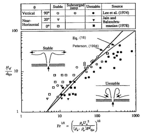

Fig. 1: Stratification criteria for round jets (PetersonPF:1994)

In case of a round buoyant plume, the criterion is the following

$$ {{4.17} \over {0.35}}\left( {{H \over {d_0 }}} \right)^{5/3} Fr_{} ^{ - 1/6} > > 1 $$

(4)

These criteria are not conditions sufficient to quantify the buoyancy gradients. It is necessary to analyse other effects in order to establish mixing or stratified conditions in enclosures: horizontal fluxes and ceiling plumes. The Rayleigh number, Ra, which is defined as

$$ Ra_H = {{g(\rho _\infty - \rho _w )H^3 } \over {\rho _\infty \nu ^2 }}\Pr $$

(5)

is used in this case to determinate these conditions. When this dimensionlessthe Rayleigh number is greaterhigher than 109, the turbulent fluxes generate density gradients which reduce the stability of the stratified layers, and poses initiates mixing patterns (WoodcockJ:2001).

Finally, the location of the release point could reduce established inhomogeneous conditions in a closed room, by the fact that the inertia forces are not enough to impulse the hydrogen below the release point. Then hydrogen will accumulate at the upper part of the room and the mixing process will be led by slower phenomena: molecular diffusion or convective heat. Some experiments as NUPEC M-8-1 (CSNI:1999) and Shebeko (ShebekoYN:1988) have illustrated this phenomenon.

References

Invalid BibTex Entry!

Influence of Natural Ventilation of Structures

In general, the accidental release of hydrogen in confined environments will be affected by ventilation streams coming from other rooms or from the atmosphere. As a general safety rule: “Any structure containing hydrogen system components shall be adequately ventilated when hydrogen is in the system” (NASA:NSS:1740:16:1997). The amount of ventilation required will vary in each case depending on the total supply of hydrogen, the rate of generation, and the venting arrangement from the process or hydrogen system. The goal of any hydrogen ventilation system is to keep the concentration below the lower flammability limit (4% at normal conditions).

Ventilation systems use vents, ducts, heat exchangers, fans and other components. They are based on the principles of natural or forced convection as described above in this chapter. Under most common conditions, hydrogen has a density lighter density than air and tends to rise upwards when in contact with air. On the other hand, the air temperature affects the ventilation behaviour: warmer air is less dense than cooler air, and therefore warm air tends to push upwards when in contact with cooler air.

The use of a fan, as a forced ventilation system, has to supply approximately 25 times the volume of hydrogen to maintain a safe concentration of hydrogen. The reliability of this system depends on the eventual event of a mechanical or electrical failure.

In order to avoid these reliability problems, passive systems are usually established on hydrogen applications in enclosures. A typical configuration is based on using high and low vents on walls. Under most common conditions, hydrogen has a lighter density than air and tends to rise upward when in contact with air. Moreover, warmer air is less dense than cooler air, and so warm air tends to push upwards when in contact with cooler air. In general, a ventilation system is driven more by air temperature differences than by hydrogen concentration, and can be affected by the difference of temperature between the enclosure and the external environment.

On a cool day, when the inside temperature is hotter than outside, the lighter warm air mixed with the lighter hydrogen in the enclosure will rise together out the high vent, drawing fresh cool air in through the low vent. Both the temperature of the warm air and the presence of hydrogen will drive the ventilation rate. Under these conditions, the hydrogen amount in the enclosure will decrease. On a warm day, the direction of air flowing through the vents can reverse. When this happens, warm air trying to enter the top vent pushes back the hydrogen trying to rise out the same vent, causing the hydrogen to stagnate and build up inside the enclosure. On this condition the hydrogen is trapped within the enclosure and the molecular diffusion is the only mechanism to mix the hydrogen. Therefore, the explosive conditions could be not avoided.

Other systems use tubes as a small chimney that catches the hydrogen at some elevation. The use of these tubes in combination with low or high vents, being set at the same height on the wall, prevents some of the unwanted thermal convection described above. However, the combination of these systems has to be studied in detail, considering the effect of the external conditions in order to avoid failures in the ventilation behaviour under certain circumstances.

References

Invalid BibTex Entry!

Experiment

Tests most representative of hydrogen behaviour within enclosures are the following:

• The Russian tests by Shebeko (ShebekoYN:1988): hydrogen distribution experiments for a subsonic release of hydrogen in a closed vessel.
• GEXCON, NH and STATOIL (GexCon:2003) performed hydrogen dispersion experiments in a confined compartmented space.
• CEA has performed slow release helium dispersion tests in their MISTRA facility, Caron-Charles and Blumenfeld (CaronCharlesM:2001), also Blumenfeld and Caron-Charles (BlumenfeldLCEA).
• Tests in the gallery facility of INERIS (LacomeJM:2007)

Aiming at the development and validation of predictive numerical tools for simulating the hydrogen and mixing processes, a valuable knowledge and experimental database has been compiledachieved in the field of nuclear fission safety through an extensive program of tests for hydrogen distribution and mixing within confined geometries, with the aim to develop and validate numerical tools for modelling hydrogen relases and mixing processes. Geometrical conditions are typical of nuclear reactor containments (large and multi-compartment), and test conditions are very nuclear-specific (high contents of steam, no venting). As an example they are worth mentioning the tests performed in the HDR and BMC facilities in Germany or the NUPEC one in Japan (CSNI:1999), as well as those planned or performed at the ThAI (KanzleiterT:2005) and PANDA (AubanO:2007) facilities.

References

Invalid BibTex Entry!

Numerical Simulations

The object of dispersion modeling of hydrogen releases is the calculation of the concentration distribution of hydrogen in their vicinity. From this distribution, envelopes of constant concentrations encompassing higher concentration levels can be determined, from which clearance distances to limit the consequences resulting form accidental ignition. The shape of these envelopes can be complex, and will depend on the emission problem, which determines the nature of the flow and its rate of release, the obstacle configurations and the environmental conditions. Computer fluid dynamics simulations are thus often used to perform such calculations, as they can take into account in principle any level of details.

---

Hydrogen Dispersion

Calculation Models for the Simulation of Atmospheric Dispersion of Gas Clouds

There are several classes of calculation models to simulate the atmospheric dispersion of gas clouds:

1. Gaussian model
2. Jet model
3. Box or slab model
4. Particle simulation model
5. k-ε model representing CFD models

The Gaussian plume model is the classical approach for the simulation of the spreading of neutral (sufficiently diluted) gases incl. pollutants or radioactivity. It is a simple model describing the concentration profile as a solution of the diffusion/advection differential equation with empirical coefficients depending on the atmospheric conditions. This model, however, is inappropriate for treating the buoyant behavior of light or heavy gases.

Dispersion models are often accompanied by a jet release model to calculate the dispersion of a released gas with significant momentum flux, which is the dominant parameter for jets. The jet can be classified into two main zones, a region of adjustment from storage conditions to atmospheric pressure and a region of ¡§conventional¡¨ jet dispersion at ambient conditions. If storage conditions are pressurized, the initial zone of adjustment will possibly include flashing for a liquid or choked two-phase jet. The conventional dispersion region begins with a so-called region of flow establishment, in which similarity profiles for the concentration and axial velocity evolve; following this the jet evolves with self-similar profiles. The main features distinguishing the various jet models are the treatment of the air entrainment and the choice of the similarity profile (e.g., top-hat, Gaussian).

The macro or two-zones mixture model developed by BASF (GiesbrechtH:1980) regards the bursting of a pressure vessel, where the high exit velocity results in a fully turbulent propagation of the vessel contents. Two zones are distinguished: a core zone of the vapor cloud where (cold) liquid droplets are still existing, and a boundary zone. In the core zone, ideal mixture with spatially constant and temporally decreasing concentration is assumed, while in the boundary zone, a spatially constant and temporally decreasing turbulent diffusion coefficient is assumed.

In box or slab models, the released gas cloud is assumed to be of cylindrical shape. The processes of advection (transport by the mean wind field), air entrainment, and gravitational spreading are implemented in empirical correlations which were derived from experiments. Box models were basically developed to simulate heavier-than-air vapor clouds with averaged temperature and concentration. In extended versions, vertical profiles of temperature and concentration can be assumed. Acknowledged box models are the US code DEGADIS (HavensJA:1990) or the British code HEGADAS (McFarlaneK:1990).

Particle simulation models are based on the stochastic nature of the movement of particles in the atmospheric wind field. In a simulation, numerous (typically 5000-15,000) particles are being emitted and their trajectories traced making a statistical analysis of the velocity fluctuations. The turbulent velocity is considered to undergo changes only after a certain time defined as the Lagrange correlation time. The distribution of the particles in a given calculation grid is then a measure for the concentration distribution. An improvement of the model is given by assuming a so-called Markov process for a particle meaning that the fluctuation part is further subdivided into a component representing the capability of remembering, and a random component. The velocity at time t is then composed of a fraction proportional to the ¡§old¡¨ velocity at time t-dt and a remainder produced in a random number generator. One representative particle simulation model is the German code LASAT (MartensR:1991).

State-of-the-art modeling of the transient behavior of gases with either positive or negative buoyancy in the atmosphere is provided by Computer Fluid Dynamics (CFD) models, which simulate complex flow processes by solving the Navier-Stokes equations in an Eulerian 3D (or 2D) calculation grid structure. This approach comprises the conservation equations of mass, momentum, and energy. Apart from being (in most cases) immensely time-consuming, these models require a detailed input of initial and boundary conditions.

In the two-equation k-ε turbulence model, special partial differential equations are solved to describe the transport of turbulence as well as its generation and dissipation. Of all the approaches, the k-ε model offers the highest relative independence of empirical relations. It appears to be the only one to allow a proper simulation of hydrogen dispersion, because it meets the requirements of describing effects such as turbulence energy in the gas cloud, interaction with the atmospheric wind field, the characteristic positive buoyancy, transient sources with initial momentum, and last but not least, gas flow in a complex geometry (buildings, terrain). K-ε modeling has been realized in a variety of computer codes distinguished by the choice of the numerical solution method, which was found to have a significant effect on the calculation procedure.

References

Invalid BibTex Entry!

Simulation in the Atmosphere

Simulation of dispersion in the Atmosphere

Only a few efforts have been made in the past to simulate the dispersion of hydrogen gas mostly due to the poor experimental data base available. Early efforts were made in the late 1970s by the Los Alamos National Laboratories on a box model for hydrogen taking into account heat transport from the ground into the cloud Invalid BibTex Entry! , and then applying the Gaussian model of neutral and buoyant dispersion as part of the WHAZAN software package (StewartWF:1990). The NASA has developed the code AFGASDM applicable to LH2 and other aviation fuels. The model is something between a Gaussian model and an Eulerian grid model solving the conservation equations following a gas ¡§parcel¡¨ released as a puff until it has diluted below the flammability limits. Effects of air entrainment and phase changes are also taken into account (BrewerGD:1981).

Simulation of dispersion in Semi-Confined Environments

A subsonic horizontal hydrogen jet experiment and subsequent CFD simulation was reported by Swain Invalid BibTex Entry! (Fig. 1 and Table 1). Hydrogen was released at 25 scf/min through a 1 cm diameter orifice. The predicted concentrations showed good agreement with measurements.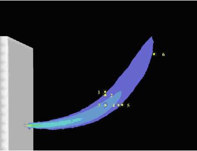

Fig. 1: Concentration contour of a 25 scf/min release. The numbers show locations where the concentration of hydrogen was measured experimentally

Table 1: Comparison between experimental and simulated H2 conc.

Sensor position	Experimental H2 conc. (%)	Simulation H2 conc. (%)	Deviation (%)
1	5.0-5.9	5.04	-8.13
2	5.6-7.0	6.96	10.48
3	9.4-10.8	13.99	38.50
4	8.1-9.4	8.25	-5.70
5	5.6-6.6	5.29	-13
6	3.5-4.6	5.37	32.60

Simulation of dispersion in Confined Environments

The use of hydrogen applications (especially automotive) in confined environments like private garages, public parking, maintenance shops, electrolysers, compressor buildings, tunnels, etc. requires detailed evaluation of the risk related to potential hydrogen leaks and if necessary identification of measures to be taken in order to avoid buildup of flammable/explosive hydrogen atmospheres. In this respect the CFD methodology has been widely used as shown in the review below, since it is generally able to realistically account for the various geometrical configurations and complex release conditions.

References

Invalid BibTex Entry!

Open Environment

The k-å atmospheric dispersion model POLLUT was used in a DLR study (EichertH:1992) to investigate hydrogen dispersion from accidental release of LH2 from vehicle tanks both in open terrain.

The computer code CHAMPAGNE was successfully applied to the NASA LH2 spill tests from 1980 (ChitoseK:1994).

(VenetsanosAG:2007)

References

Invalid BibTex Entry!

Urban Environment

The BAM 5 and 6 LH2 dispersion experiments in the presence of buildings Invalid BibTex Entry! were simulated by (StatharasJC:2000) using the ADREA-HF code. The source was modelled using a series of two phase flow jets. Liquid phase evaporation during the dispersion was taken nto account using the homegeneous equilibrium model. The calculations were performed using a one-equation turbulence model. Reasonable agreement with measured concentrations was reported when ground heating was taken into account.

The Battelle k-å model BASSIM originally designed for hydrogen combustion in nuclear containments has been applied to predicting the BAM LH2 release trials in 1994, providing reasonable qualitative results for 3D effects of hydrogen dispersion behavior (RastogiAK:1994).

The 1983 Stockholm (Sweden) hydrogen accident was simulated by Venetsanos et al. (VenetsanosAG:2003) using the ADREA-HF code for dispersion and the REACFLOW code for the combustion. An intergal tool was applied to simulate the release of 4kg of hydrogen from a network of 18 interconnected cylinders of 15 l volume each containing hydrogen at 200 bar. Figure 1 shows the predicted lower flammability (4%) hydrogen-air cloud at 10 seconds after start of release.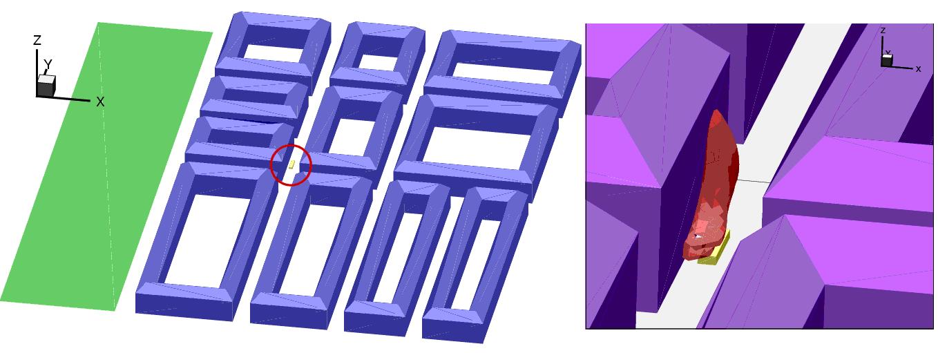

Fig. 1: Simulation of the 1983 Stockholm hydrogen accident (VenetsanosAG:2003), Left: Modelled site and lorry carrying 4 kg of hydrogen in 18x50 l, 200 bar bottles (red circle), Right: Predicted lower flammability hydrogen-air cloud at 10 seconds after start of release

Simulations of hydrogen releases from CGH2 commercial vehicles (busses) in urban environment were reported by (VenetsanosAG:2008). The work was performed during the EIHP2 project (EIHP:url), using the ADREA-HF code for dispersion and the REACFLOW code for combustion. Three different storage pressures were considered for the CGH2 releases 200, 350 and 700 bar. Compartive simulations were performed for a 200bar CNG bus.

References

Invalid BibTex Entry!

Tunnels

The k-å atmospheric dispersion model POLLUT was used in a DLR study (EichertH:1992) to investigate hydrogen dispersion from accidental release of LH2 from vehicle tanks in a road tunnel.

Simulations of hydrogen releases from LH2 and CGH2 private vehicles (cars) in a naturally ventilated tunnel were reported by Wilkening et al. (WilkeningH:2000). The work was performed within the framework of the EIHP project (EIHP:url). The ADREA-HF code was used for the dispersion calculations. The REACFLOW code was used for the combustion calculations. Two LH2 release scenarios were considered. A flow restrictor installed and a two-phase release of 8.3 g/s was assumed in the first scenario. A shut-off valve activated 5 seconds after the release and a gaseous release of 60g/s was considered in the second. For the CGH2 scenario sonic release from a 200bar storage tank was assumed. The reported overpressure results indicated that for the scenarios considered there is no major difference in using liquid hydrogen or compressed hydrogen fuel.

Tunnel accidents with an LH2 powered vehicle were simulated by Breitung et al. (BreitungW:2000). The investigated scenarios assume damage of the LH2 system, release of gaseous hydrogen, mixing with air, ignition and finally combustion. Calculations showed that gaseous hydrogen rises to the tunnel ceiling forming a strongly stratified mixture. Shape, size, inner structure and temperature of the evolving H2-air cloud were calculated. Using new developed criteria, the time and space regions with potential for fast combustion modes were identified. For the given hydrogen sources the combustion regime is governed by the ignition time. For late ignition a slow and incomplete combustion of the partly premixed H2-air cloud along the tunnel ceiling was predicted. For early ignition a standing diffusion flame develops with dimensions and heat fluxes determined by the hydrogen release rate. Temperature, oxygen and flow velocity fields during the combustion were computed. In both cases only minor pressures were generated. The highest damage potential appeared to exist for intermediate ignition times.

Simulations of hydrogen releases from CGH2 commercial vehicles (busses) in tunnel environment were reported by (VenetsanosAG:2008). The work was performed during the EIHP2 project (EIHP:url), using the ADREA-HF code for dispersion and the REACFLOW code for combustion. Three different storage pressures were considered for the CGH2 releases 200, 350 and 700 bar. Compartive simulations were performed for a 200bar CNG bus.

CFD simulations of hydrogen dispersion in tunnels was performed by (MukaiS:2005), using the STAR-CD code and standard k-ε model. The amount of hydrogen leaked was 60 m3 (approximately 5.08 kg), which corresponds to the amount necessary for future fuel cell vehicles to achieve their desired running distance. The study considered the typical longitudinal and lateral areas of tunnels, the undergound ventilation facilities and the electrostatic dust collectors.

References

Invalid BibTex Entry!

Residential Garages

Hydrogen leaks inside a residential garage compared against gasoline, natural gas and propane leaks in the same environment were simulated by Swain (SwainMR:1998) using the FLUENT code. Calculations were based on the GEOMET Invalid BibTex Entry! garage geometry (2.52x6.59x2.74 m) with a single vent placed in the center of one wall of an otherwise sealed garage. The leak rates for fuels other than hydrogen were adjusted for equal size holes and equal energy flow rates in the fuel lines considering both laminar and turbulent flow where applicable. The results of the simulations show that for the lower leakage rate (1000 l/hr) and typical garage air exchange (2.92 ACH representing natural ventilation), hydrogen and methane did not create dangerous conditions while propane and gasoline did produce dangerous conditions in similar accident scenario. For the larger fuel leakage rate (7200 l/hr) and minimal air exchange rate (0.2 ACH) all four fuels produced very large combustible clouds after 2 hours of leakage. However, the energy content of the combustible clouds was different, with hydrogen being at most % that of the other fuels. Both natural gas and hydrogen filled the entire garage with a flammable mixture after two hours, while propane and gasoline filled just over half of the garage volume with a flammable mixture. At the higher air exchange rate (2.92 ACH), the hydrogen still filled the garage with a flammable mixture, which reached about 6.6% hydrogen concentration after two hours.

Boil-off from the cryogenic hydrogen tank of a car in a private garage was simulated by Breitung et al. (BreitungW:2000) using the GASFLOW code to calculate the temporal and spatial distribution of hydrogen and criteria to evaluate the flame acceleration and detonation potential. Boil-off was assumed occurring at a rate of 170 g day-1 and the boil-off release to occur intermittently in five pulses per day of 100 or 10 s time period each, which gave 0.34 or 3.4 g s-1 respectively.

CFD modelling (FLUENT) was used in Invalid BibTex Entry! to analyze H2 leak scenarios inside residential two vehicle garages. The study was based on parking a 5-passenger sedan with compressed H2 gas reservoir carrying capacity of 6 kg at 10,000 psi (689.5 bar) pressure. The HFCV was designed to comply with SAE J2578 and J2579 standards for H2 and fuel cells, which include provisions for safety systems onboard the vehicle. Such assumed mechanisms include the implementation of a hydrogen detector in each wheel well. Each detector was designed to signal a shut down and isolation H2 procedure upon detecting 1% H2. Another assumed mechanism includes the use of an on-board computer that is capable of shutting down H2 flow upon detecting a larger than 20 CFM leak (9.4 lt s-1) when the vehicle is dormant. In addition the HFCV was equipped with a valve that isolates H2 in the tank upon engine (fuel cell) shut down. This assumed isolation mechanism was designed to monitor and test for leaks upon vehicle shutdown and prior to start up by the on-board computer. In the study most of the modelling scenarios were based on a 20 CFM leak from beneath the vehicle. This leak rate corresponded to a fuel cell power output of about 50 kW. It was found that for the considered garage layout and scenarios no modifications to the baseline structures would appear to be necessary for vehicles equipped with safety systems that detect hydrogen leaks according to the chosen scenarios. CFD modelling of one configuration showed that a 1% hydrogen concentration would reach the wheel well within 28 seconds where detectors could initiate a shut off of the fuel supply. Since not all vehicles will be equipped with hydrogen detectors, or be configured like the chosen vehicle design, additional modelling provided data on the time for a 5% hydrogen concentration to accumulate at the garage ceiling. This information may be used by carmakers to develop strategies to limit the amount of time that the vehicle operates at zero speed before shutting off the fuel supply.

(GallegoE:2005)

Helium dispersion experiments in a private garage including a mockup of a car and performed by Swain Invalid BibTex Entry! were simulated by Papanikolaou and Venetsanos (PapanikolaouEA:2005) using the ADREA-HF code and the standard k-å model. Helium was released below the car at a flow rate of 7200 l/hr. The predicted results were found generally in acceptable agreement with the experiment. For the case with the lowest vent size the vertical concentration gradient was found underestimated compared to the experiment. This was attributed to the turbulence model overestimating mixing under the given low flow conditions.

References

Invalid BibTex Entry!

Maintenance Shops

CFD modelling (FLUENT) was used in Invalid BibTex Entry! to analyze H2 leak scenarios inside a commercial maintenance/repair/service station. The study was based on a 5-passenger sedan with compressed H2 gas reservoir carrying capacity of 6 kg at 10,000 psi (689.5 bar) pressure. The HFCV was designed to comply with SAE J2578 and J2579 standards for H2 and fuel cells, which include provisions for safety systems onboard the vehicle. Such assumed mechanisms include the implementation of a hydrogen detector in each wheel well. Each detector was designed to signal a shut down and isolation H2 procedure upon detecting 1% H2. Another assumed mechanism includes the use of an on-board computer that is capable of shutting down H2 flow upon detecting a larger than 20 CFM leak (9.4 lt s-1) when the vehicle is dormant. In addition the HFCV was equipped with a valve that isolates H2 in the tank upon engine (fuel cell) shut down. This assumed isolation mechanism was designed to monitor and test for leaks upon vehicle shut down and prior to start up by the on-board computer. In the study most of the modelling scenarios were based on a 20 CFM leak from beneath the vehicle. This leak rate corresponded to a fuel cell power output of about 50 kW. For the considered maintenance facility and scenarios no modifications to the baseline structures were recommended. The high rates of ventilation would dilute the assumed 20-CFM leak and result in a flammable mixture only in close proximity to the vehicle. The potential for flammable mixtures forming at the ceiling of the facility was assessed. The time required for a hydrogen leak to result in 20% of LFL at the ceiling was determined for different vehicle leak rates. Options for improving the ventilation in the building were presented.

References

Invalid BibTex Entry!

Public Parking

CFD modelling (FLUENT) was used in Invalid BibTex Entry! to analyze H2 leak scenarios inside a commercial multi-story above-ground parking and a commercial multi-story below-ground parking. The study was based on parking a 5-passenger sedan with compressed H2 gas reservoir carrying capacity of 6 kg at 10,000 psi (689.5 bar) pressure. The HFCV was designed to comply with SAE J2578 and J2579 standards for H2 and fuel cells, which include provisions for safety systems onboard the vehicle. Such assumed mechanisms include the implementation of a hydrogen detector in each wheel well. Each detector was designed to signal a shut down and isolation H2 procedure upon detecting 1% H2. Another assumed mechanism includes the use of an on-board computer that is capable of shutting down H2 flow upon detecting a larger than 20 CFM leak (9.4 lt s-1) when the vehicle is dormant. In addition the HFCV was equipped with a valve that isolates H2 in the tank upon engine (fuel cell) shut down. This assumed isolation mechanism was designed to monitor and test for leaks upon vehicle shut down and prior to start up by the on-board computer. In the study most of the modelling scenarios were based on a 20 CFM leak from beneath the vehicle. This leak rate corresponded to a fuel cell power output of about 50 kW. For the considered below and above ground parking facilities and scenarios no modifications to the baseline structures were recommended. Existing ventilation in the below ground structure would dilute a 20-CFM hydrogen leak so that a flammable mixture would only exist in close proximity to the vehicle. Similarly, natural ventilation would dilute hydrogen leaks for the above ground parking facility.

References

Invalid BibTex Entry!

Hydrogen Refuelling Stations

High pressure hydrogen release experiments inside the storage room of a full scale model of a hydrogen refueling station were reported by Tanaka et al. (TanakaT:2005). Storage pressure was 40 MPa while nozzle diameters in the range 0.8-8 mm. The storage room with dimensions 6x5x4 m included 35 cylinders of 250 l capacity each. Ventilation openings of 1m height existed on all 4 sidewalls and where either 50% or 100% open. The time history of the average hydrogen concentration in the room was modelled usimg a simple gas accumulation model (CleaverRP:1994) and compared against the experimental data. It was found that the model is able to predict well the experimental concentrations in the experiments involving more slowly varying pressure (lower nozzle diameters), but tends to overpredict the concentrations for the higher nozzle diameter.

References

Invalid BibTex Entry!

Other Applications

Hydrogen dispersion experiments in a half-scaled hallway and subsequent CFD validation using the FLUENT code were performed by Swain (SwainMR:1999). Hydrogen leaked at a rate of 2 SCFM (0.94 lt/s) from the floor at the left end. At the right end of the hallway, there were a roof vent and a lower door vent for the gas ventilation. Four sensors were used to record the local hydrogen concentration variations with time. Predicted hydrogen concentrations time series were found in good agreement with the experimental data. The same experiments were simulated by Agranat et al. {[DB, AgranatV:2004]], using the PHOENICS code. Predicted results were found similar to the ones obtained using the FLUENT code with maximum concentration differences between the two models of about 20%.

Catastrophic hydrogen releases inside the Alpha H2BPS (H2 Backup Power System by Stewart Energy) generator room were simulated by Agranat et al. (AgranatV:2004) under real industrial working scenarios and real geometry, using the PHOENICS code and the LVEL turbulence model. Two scenarios were considered in the simulations: a vertical fast release from a high-pressure line and a horizontal fast release from a medium-pressure line. The CFD simulations showed that the two installed sensors are capable of detecting 10% LFL cloud (0.41%) separately at 8.8 and 9.7 seconds for the high-pressure vertical leak, but only one sensor which is closer to the leak orifice can detect the same concentration cloud within 20 seconds for the medium-pressure horizontal release. The numerical simulation confirmed that the current sensor installation can promptly report the potential catastrophic hydrogen leak under the above scenarios. However, the fact that 10% LFL hydrogen cloud cannot reach one sensor during the horizontal release indicates that the sensor location can be further optimized and more sensors are required for the systems.

The method for determination of maximum ventilation described in the standard IEC EN 60079-10 was validated by Nilsen et al. (NilsenS:2004) for a small hydrogen production (by water electrolysis) unit located inside two different enclosure geometries, using the FLACS code for dispersion and the PHAST code for release. It was found that the model suggested in standard IEC EN 60079-10 is not a conservative approach when deciding the ventilation capacity large enough to keep flammable gas clouds at a negligible size and therefore must be used with care.

References

Invalid BibTex Entry!

Knowledge Gaps and Recent Progress

Simulations of hydrogen dispersion using the CFD methodology have increasingly grown in number during the last 10 years and are expected to grow even more in the near future. Prediction of the time and space distribution of the flammable hydrogen clouds evolving after accidental hydrogen leaks of various types in widely different environments is the main output necessary for subsequent risk assessment estimation of the various hydrogen applications. In this process, simulations have been performed using different CFD codes (commercial or research tools) and different modelling strategies (turbulence models,source treatment, discretization options, etc.).

To ensure the quality and trust in industrial CFD applications best practice guidelines have been developed in the past either of a general character like ERCOFTAC 2000 (CaseyM:2000) or more related to particular applications like HSL 2003 Invalid BibTex Entry!. No CFD guidelines specific to hydrogen dispersion applications have been proposed.

Taking the above in consideration a significant effort has been concentrated within the European Network of Excellence HYSAFE with aim to perform a systematic evaluation of the various CFD approaches (codes and models) in predicting hydrogen dispersion, based on a series of benchmark exercise problems, using existing and new state of the art experimental data.

The results of the first such hydrogen dispersion benchmark exercise (SBEP-V1) were reported by Gallego et al. (GallegoE:2005). The experiment simulated was that of Shebeko et al. (ShebekoYN:1988), who investigated the dispersion of hydrogen in an hermetically closed cylinder (20m3 volume) by measuring axial hydrogen concentrations (6 locations) at times from 2 to 250 minutes following an initial 60 s vertical subsonic jet release at a rate of 4.5 l/s from a 10mm nozzle. Large variations in predictions were monitored during this first benchmark (as expected), which could be attributed to variations in turbulence models, boundary conditions as well as discretization options.

The aim of the second hydrogen dispersion benchmark exercise (SBEP-V3) was three fold a) to further investigate on the ability of the models to predict the long term stratification/diffusion problem in a confined space, b) to test the ability of models to predict the concentration field of a vertical subsonic hydrogen jet release and c) to attempt to minimize or justify large variations between model predictions. Newly performed hydrogen dispersion experiments by INERIS at their gallery facility (garage like enclosure with dimensions 7.2x3.8x2.9 m) were used for this benchmark. The release was vertical upwards at a rate of 1 g/s from an orifice of 20 mm diameter and lasted for a period of 240 s. The total simulation time was 5400 s. The benchmark took part in two phases a blind pre-test phase and a post–test one.

Further benchmarks focus on testing the ability to predict free choked hydrogen flows, obstacle effects on hydrogen dispersion within confined spaces as well as hydrogen dispersion from LH2 releases.

Computer fluid dynamics simulations of chocked flows are difficult to tackle due to the presence of the shock waves. The simulations may require, for commercial solvers, resolving the Mach cone and the shock wave patterns to some degree of details. Since the extent of the flammability envelopes resulting from chocked releases from apertures of about 1 cm may reach 10 to 100 m depending on the storage pressure, length scales of up to five orders of magnitude must be covered by the mesh. In addition, convergence will usually be problematic.

The difficulties faced by direct CFD simulations of chocked releases may be alleviated by using effective diameter approaches/ The applicability of effective diameter approaches to horizontal releases of hydrogen should be investigated further, particularly for the large hydrogen releases resulting from high pressure flows, where the effects of buoyancy on the shape of the release remain an issue.

For choked hydrogen releases the fact that the molar concentration is proportional to the inverse distance has been observed experimentally, but given that significantly different proportionality constants have been reported, a systematic investigation both experimental and computational is still required to cover a wider range of storage pressures and orifice diameters.

Regarding obstacle effects on hydrogen dispersion it should be mentioned that steady-state flow rates can lead to unsteady behaviour of the dispersion pattern in some cases, particularly when impingement flows or external flows (over a surface) are considered, due to significant vortex shedding. Such situations may require a statistical definition of the constant (flammable) concentration envelope, based on the probability distribution of finding a given concentration of hydrogen at a specific location at a given time.

Finally as far as LH2 release and dispersion are concerned it seems that more experimental information is needed to trigger further physical understanding and model development/improvement. From the past experience it seems that these proposed tests should focus on better control over the experimental conditiosn (less uncertainty).

References

Invalid BibTex Entry!

---

Hydrogen Dispersion